
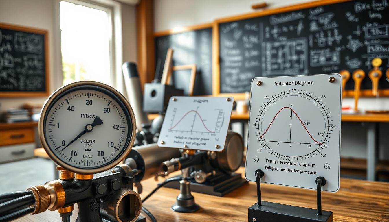
Have you ever wondered if we could see thermodynamic work in real-time? Not in textbooks, but in the real world of a steam engine. It’s a messy, beautiful sight.
An indicator diagram is like a machine’s EKG. It shows the mechanical work as it happens. The Victorians created this tool when “data visualization” meant actual ink on paper.
The PV curve reveals the mean effective pressure on your piston. It shows your engine’s power, valve performance, and exhaust. It also tells if you’re using the right amount of steam. Just like converting water to watts, it turns abstract thermodynamics into real power.
This project teaches you to make your own pressure-volume analysis. It uses modern sensors and microcontrollers. Learning from the gap between reality and theory is valuable.
Low cost setup Arduino ESP32 pressure sensor rotary encoder
Imagine telling a Victorian steam engineer about measuring cylinder pressure with $50 electronics. They’d think you’re crazy. Those old mechanical indicators were pricey, with springs and precision machining.
Today, we have the ESP32 microcontroller at the heart of our system. It’s like Arduino’s high-tech cousin, with dual cores and WiFi. It handles data fast, turning analog signals into digital data quickly.
We use piezoresistive sensors for cylinder pressure, in the 0-200 PSI range. These sensors cost under $30. They connect to the cylinder head, where old indicators used to be.
The rotary encoder tracks the piston’s position. It mounts on the crankshaft, sending pulses as it rotates. You can choose between optical encoders for precision or Hall effect sensors for simplicity.
Modularity is key here. Each part does one thing:
| Component | Function | Output Signal | Typical Cost |
|---|---|---|---|
| ESP32 Board | Data acquisition and processing | Digital via USB/WiFi | $8-12 |
| Piezoresistive Sensor | Cylinder pressure measurement | 0-5V analog | $25-30 |
| Rotary Encoder | Crankshaft position tracking | Digital pulses | $10-15 |
| Breadboard & Wires | Component interconnection | Electrical pathways | $8-12 |
| Power Supply | System power regulation | 5V DC regulated | $6-10 |
Your total cost is between $50 and $80, depending on what you already have. Commercial engine indicators cost thousands. We’re making lab-grade tools for less than a tank of gas.
The ESP32 reads the pressure sensor and counts encoder pulses in real time. It does this without any special interfaces. You control everything with your code.
Old methods used oscilloscopes or PC systems like Labview. But our ESP32 setup is cheaper and gives you more control. This is important for machines that are hard to measure.
Today, electronics are more accessible. We can make complex systems with just a few parts. All you need is curiosity and basic skills to start building.
Calibration absolute vs gauge zero drift sampling rate
Before you can draw a meaningful indicator diagram, you need to confront an uncomfortable truth about pressure sensors. Most affordable sensors report gauge pressure, which is pressure relative to the surrounding atmosphere. This creates a problem when trying to capture the complete thermodynamic story of your steam engine’s cycle.
Your sensor might show zero PSI when the cylinder sits at atmospheric pressure. But from a thermodynamic perspective, there’s 14.7 PSI of absolute pressure doing real work at sea level.
That offset matters a lot when calculating actual work output. The Victorian engineers who developed the original indicator diagram methodology understood this. They established what they called the “vacuum line,” a zero absolute reference from which all meaningful pressure measurements must originate.
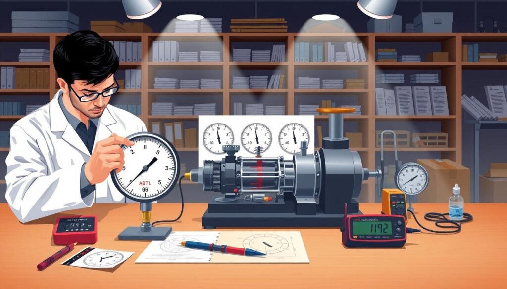
Atmospheric pressure is your frenemy. It changes with weather patterns and altitude. So, that canonical 14.7 PSI is really more of a suggestion than a constant. If you’re running your model engine in Denver, you’re starting from roughly 12.1 PSI atmospheric.
You have two choices: install a separate barometric pressure sensor for real-time atmospheric correction, or measure local atmospheric pressure once and accept minor variations. For hobbyist-level accuracy, the second approach works fine—we’re not calibrating NASA equipment here.
Then there’s zero drift, that sneaky phenomenon where your sensor’s baseline reading wanders. This can be due to temperature changes, mechanical stress, or what I like to call the sensor’s existential uncertainty about its purpose. Modern piezoelectric and MEMS sensors are prone to thermal drift. As the engine heats up, the sensor’s zero point can shift by several PSI, corrupting all your subsequent readings.
The practical solution is refreshingly straightforward. Take a zero reference reading before each measurement run when the cylinder is at atmospheric pressure and the engine is at operating temperature. Subtract that offset from all subsequent readings during data acquisition.
This technique compensates for both thermal drift and any mounting stress effects. It’s not elegant, but it works—which describes most good engineering practices.
| Measurement Type | Reference Point | Typical Reading at Atmosphere | Best Application |
|---|---|---|---|
| Gauge Pressure | Local atmospheric pressure | 0 PSI | Pressure differentials, simple monitoring |
| Absolute Pressure | Perfect vacuum | 14.7 PSI (sea level) | Thermodynamic calculations, PV diagrams |
| Gauge + Atmospheric Offset | Calculated absolute | Varies with altitude/weather | Hobbyist indicator diagrams |
Sampling rate deserves its own meditation session. Too slow, and you miss the critical rapid pressure changes at cutoff and release points. Too fast, and you’re drowning in redundant data while your microcontroller chokes on buffer overflow.
For model steam engines running at 500-2000 RPM, you want at least 100 samples per revolution. Ideally, aim for 200-360 samples to capture one pressure reading per degree of crank rotation. The math is simple: at 1000 RPM, that’s 16.67 revolutions per second, requiring 3,333 to 6,000 samples per second.
Fortunately, the ESP32’s ADC can handle sampling rates up to several hundred kHz, so we’re not hardware-limited. The real constraint is matching your sampling rate to encoder resolution and keeping data arrays manageable in RAM. A 360-sample buffer per cycle at 4 bytes per sample consumes only 1.4 KB—trivial for modern microcontrollers.
Now, about calibration rigor. One source mentions constructing a precision calibration rig resembling a “piston-phone”—a device used for microphone calibration with sub-millimetric displacements and deeply sub-Pascal pressures. That’s theoretically correct but practically absurd for our purposes.
We’re measuring steam engine performance, not calibrating NIST reference standards. A simpler approach yields perfectly adequate results: verify your pressure sensor against a known accurate mechanical gauge at two or three pressure points across your expected operating range. Most decent sensors exhibit sufficient linearity that a two-point calibration (atmospheric and one elevated pressure) gets you within 2-3% accuracy.
That’s frankly better than the Victorian engineers managed with their mechanical spring-loaded indicators, and they built empires with those instruments. Sometimes good enough really is good enough—when the alternative is analysis paralysis preventing you from collecting any data at all.
Acquire one cycle data sync pressure with crank angle
Getting data without timing is like taking photos with your eyes closed. You might get something, but it won’t make sense. The key to useful data is synchronization. You need to know the exact piston position for each reading.
Your rotary encoder becomes the leader of your measurement team. It sends pulses as the crankshaft moves. By counting these, you link each pressure reading to a specific crank angle. This method works no matter the engine speed.
Whether the engine is slow or fast, you get the same detail. The encoder’s pulse count stays the same, keeping your data consistent.
Finding the right start time is the big challenge in data acquisition. You need a clear start point, like Top Dead Center (TDC). This can be found with an encoder pulse or a Hall sensor.
When the ESP32 finds this point, it starts filling an array with pressure-angle pairs. It’s like a dance, with each step showing a different angle and pressure.
At high engine speeds, regular checks won’t work. Your code needs to be interrupt-driven. Missing a pulse messes up your angle calculations.
Now, you have to decide: capture one perfect cycle or average many? Each method shows different engine performance truths.
| Acquisition Method | Advantages | Disadvantages | Best Use Case |
|---|---|---|---|
| Single-Cycle Capture | Raw, unfiltered reality; reveals instantaneous behavior; detects anomalies | Includes all noise and irregularities; less representative of typical operation | Troubleshooting, peak performance analysis, detecting misfires |
| Multi-Cycle Averaging | Smooths random variations; more representative diagram; cleaner curves | Hides cycle-to-cycle variations; masks intermittent problems | Calculating work per cycle, steady-state performance mapping |
| Overlaid Multiple Cycles | Shows consistency and variation simultaneously; diagnostic power; visual appeal | Requires more memory and processing; complex display logic | Professional analysis, engine health assessment, detailed diagnostics |
I suggest capturing both. Get 10-20 cycles and show them together. This lets you see both consistency and variation. Then, show the average for a clearer picture.
For engines that work in both directions, you need measurements from both ends. This is best done with two sensors. If not, measure one end at a time.
Your code should be simple. Use two arrays: crankAngle[360] and cylinderPressure[360]. These are filled during each revolution, ready for analysis.
For reliable synchronization, your interrupt service routine (ISR) must be efficient. It should quickly read the sensor and store the value. Leave the heavy work for your main loop.
Remember, let your engine warm up before serious data capture. Cold engines behave differently than hot ones. You want data from the engine’s real operating conditions.
Convert to volume using bore stroke clearance volume
You’ve got pressure readings synced to crank position, but now comes the critical step: calculating what volume corresponds to each angle. This conversion transforms raw data into something thermodynamically meaningful. It’s where your measurements become an actual indicator diagram.
Start with the basics: your engine’s bore and stroke define the swept volume. The bore is the cylinder diameter, and the stroke is how far the piston travels. For a cylindrical volume, the math is straightforward: π × (bore/2)² × stroke gives you the total volume displaced in one complete stroke.
But there’s a catch that trips up beginners every time. Volume doesn’t hit zero when the piston reaches Top Dead Center. There’s always clearance volume—the space between the piston face and cylinder head at the end of compression, including ports, passages, and steam chest volume.
How much clearance should you expect? It varies significantly based on engine design. Slow-speed, long-stroke engines typically run 2-4% clearance relative to swept volume. High-speed, short-stroke engines might push 8% or higher.
| Engine Type | Speed Characteristic | Typical Clearance | Design Consideration |
|---|---|---|---|
| Slow-speed stationary | Long stroke | 2-4% | Maximum expansion efficiency |
| Medium-speed marine | Moderate stroke | 4-6% | Balance of power and durability |
| High-speed model | Short stroke | 6-8% | Higher RPM capability |
| Racing configuration | Very short stroke | 8-10% | Peak power at high RPM |
Measuring clearance volume requires patience. One proven method: fill the clearance space with liquid from a graduated cylinder when the piston sits at TDC. For model engines with complex porting, you might calculate it from technical drawings or estimate based on similar engines.
Now comes the geometry. The piston doesn’t move linearly as the crank rotates—it follows a sinusoidal pattern modified by connecting rod length. For a slider-crank mechanism, piston position as a function of crank angle θ involves both crank radius r and connecting rod length L.
The complete formula looks like this: position = r×(1-cos(θ)) + L×(1-sqrt(1-(r/L×sin(θ))²)). That square root term accounts for the connecting rod’s angular motion. If your connecting rod is long relative to crank radius—typical ratio is 4:1 or better—you can simplify with an approximation: position ≈ r×(1-cos(θ)).
Converting position to volume follows logically. Multiply piston position by piston area to get displaced volume. Add your measured clearance volume to that result. Suddenly you’ve transformed your crank angle array into a cylinder volume array.
Here’s your conversion checklist:
- Calculate swept volume from bore and stroke measurements
- Measure or estimate clearance volume for your specific engine
- Apply slider-crank formula to convert each crank angle to piston position
- Multiply position by piston area, then add clearance volume
- Verify minimum volume equals clearance and maximum equals clearance plus swept volume
That verification step isn’t optional—it’s critical. If your calculated minimum doesn’t match measured clearance, you’ve got an error somewhere in the conversion chain. Same goes if maximum volume doesn’t equal clearance plus swept volume. Garbage in, garbage out, as they say in data processing circles.
Now you’ve got matching pressure and volume data points. This is exactly what you need to plot a proper PV curve. The area inside that curve represents work per cycle, and if your volume scale is wrong, your work calculation will be proportionally wrong.
The beauty of this conversion is how it bridges measurement and theory. You started with sensor voltages and encoder pulses. Now you’re holding thermodynamic data that reveals how efficiently your engine converts heat into mechanical work. That’s the kind of mathematical handshake that makes engineering projects worthwhile.
Plot PV compute loop area work per cycle then power work × rpm
Now, let’s see the results: plotting the pressure-volume relationship and finding the work per cycle your engine does. This turns all your measurements into real mechanical energy. The indicator diagram you’ll make looks like something a Victorian engineer would know well.
Making the PV curve is easy. Just put pressure on the Y-axis and volume on the X-axis. Your data points will form a closed loop. With Python and matplotlib, it takes just a few lines of code. Or, you can watch it draw on an ESP32 TFT screen in real-time.
The curve’s shape shows if everything is working right. You should see a rectangular loop with curved corners. The admission line goes up sharply as steam enters, then stays flat during admission.
It curves down during expansion. The pressure drops at release, stays flat during exhaust, and goes up slightly during compression. If your loop looks like art or crosses itself, there’s a problem with your measurements or engine timing.
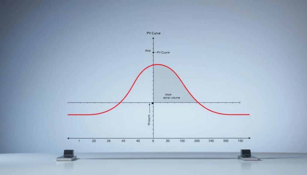
The area inside the loop is the work per cycle. This is the energy taken from steam in one full cycle. There are old ways and new ways to calculate this area.
The old way used the “method of ordinates.” It divided the diagram into parts, measured pressure, and averaged those to find Mean Effective Pressure. Then, it multiplied by swept volume.
The planimeter method used a mechanical device to measure area. Today, we use numerical integration, like the trapezoidal rule, on your pressure-volume data. This is quick and accurate.
The area you find has units of pressure times volume, which equals energy. If your units are PSI and cubic inches, you get inch-pounds. Divide by 12 for foot-pounds. From work per cycle, you can find power output by multiplying by RPM divided by 60.
The classic formula for indicated horsepower also gives you the same power. It multiplies MEP by piston area, stroke length, and RPM, then divides by 33,000. This converts foot-pounds per minute to horsepower. Both methods should match if your math is correct.
| Calculation Method | Input Parameters | Best Use Case | Accuracy Level |
|---|---|---|---|
| Numerical Integration | P-V data arrays | Digital systems with continuous sampling | High (±2%) |
| Method of Ordinates | 10 pressure measurements at equal volumes | Manual plotting or sparse data | Medium (±5%) |
| MEP Formula | Average pressure, bore, stroke, RPM | Quick estimates and validation | High if MEP accurate |
| Planimeter | Physical diagram on paper | Historical methods or verification | Medium (±4%) |
Show off your result: “Indicated Power: 0.12 HP at 1500 RPM” is much more satisfying than just seeing lines. You’ve made the invisible visible. You’ve measured what the Victorians did with brass and mahogany, but with silicon and code.
For extra credit, calculate thermal efficiency by comparing this work to the steam’s enthalpy drop. You’ll likely get something low, like 5-8% for a simple model engine. That’s not an error—it’s thermodynamics telling you that entropy wins and the universe always takes its share.
The power output calculation checks everything before it. If your numbers seem too high, check your pressure. Too low? Look at your volume or RPM. The indicator diagram shows reality with math precision.
Error analysis lag filtering smoothing uncertainty bars
Every sensor has some error, like a car with a check engine light that keeps running. Your pressure sensor has noise, and your rotary encoder has jitter. Measurement uncertainty is just physics showing us that perfection is only in textbooks.
It’s not about if you have errors, but if you understand them well enough to trust your results.
Sensor lag is the first issue. Most pressure sensors take milliseconds to respond. At 300 RPM, your engine does one full revolution in 0.2 seconds. If your sensor has a 5-millisecond lag, that’s about 9 degrees of crank rotation between when pressure changes and when your data system records it. This creates a phase shift that makes your indicator diagram look rotated or warped.
The sharp pressure drop at cutoff might appear several degrees late. The compression curve could be shifted rightward on your plot.
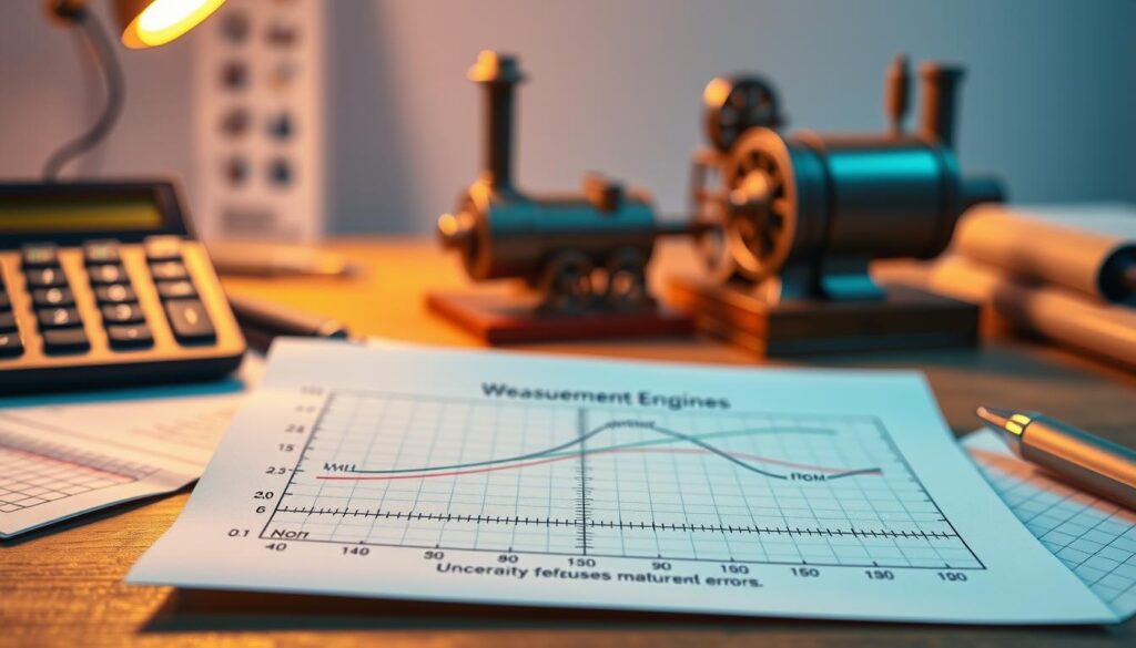
You can correct for this by characterizing your sensor’s response time and applying a phase correction to your data. Or you can acknowledge the limitation and stick to lower RPM ranges where the lag is negligible compared to cycle duration. Either approach works, but pretending the lag doesn’t exist doesn’t.
Signal filtering is a delicate balance. Too much smoothing and you’ll erase real features like the cutoff spike. Too little and your PV curve looks like it was sketched during an earthquake. A moving average filter with a 3-5 sample window often strikes the right balance for steam engine data acquisition.
For those who enjoy mathematics, a low-pass digital filter works even better. Set the cutoff frequency just above your fundamental engine frequency to preserve cycle features while rejecting high-frequency noise.
Here’s the golden rule: always show both raw and filtered data. This lets you verify the filtering isn’t creating artifacts or hiding real behavior.
| Error Type | Typical Magnitude | Detection Method | Correction Strategy |
|---|---|---|---|
| Sensor lag phase shift | 5-15 degrees at high RPM | Compare cutoff timing to valve events | Apply calculated phase correction or reduce RPM |
| Random noise cycle variation | ±2-5% peak pressure | Standard deviation across multiple cycles | Average 10-20 cycles and plot uncertainty bars |
| Systematic pressure offset | ±1-3% absolute reading | Compare calculated MEP to theoretical values | Recalibrate sensor or apply known correction factor |
| Crank angle zero drift | ±3-8 degrees TDC reference | Verify compression TDC matches mechanical TDC | Adjust trigger position or software offset |
Uncertainty bars on an indicator diagram are rare but informative. If you’re averaging multiple cycles, plot the standard deviation as error bars at 8-10 representative points around the loop. Tight error bars mean consistent operation. Large error bars indicate cycle-to-cycle variation from timing issues, valve leakage, or load fluctuations.
I’ve seen diagrams where the expansion curve had error bars ±15% of the mean pressure. That’s not a measurement problem—that’s the engine telling you something is mechanically wrong.
Systematic errors are sneakier than random noise because they don’t show up in repeatability tests. Is your pressure sensor reading consistently 2% high? Is your crank angle zero reference actually 5 degrees off from true top dead center? These errors will skew your absolute measurements while your cycle-to-cycle variation looks perfectly acceptable.
The solution is independent verification. Calculate expected MEP from your steam inlet conditions and compare it to measured MEP. Benchmark against published data for similar engines. As one Victorian-era engineer noted, interpreting diagrams requires “careful study and discriminating judgment”—which translates from 19th-century speak as “don’t just trust the numbers; think about whether they make physical sense.”
If your calculated power output exceeds the theoretical maximum efficiency of a Carnot cycle operating between your steam and exhaust temperatures, you’ve either revolutionized thermodynamics or made a math error. I’m betting on the latter.
Historical engineers understood this intuitively. They knew that “the only absolute information a diagram gives is the varying pressure of the steam in the cylinder.” Everything else—power calculations, efficiency estimates, comparative analysis—requires careful error analysis and an honest accounting of what you can and cannot measure with confidence.
The best practice? Document everything. Note your sensor specifications, sampling rates, filtering parameters, and calibration methods. When you publish your results, include measurement uncertainty estimates. Future you, looking back at old data, will thank present you for the honesty.
Compare throttled vs wide open curves pumping loss talk
Looking at PV curves side by side shows the cost of throttling. It’s like watching money vanish. Run your steam engine at full throttle and capture an indicator diagram. Then, throttle it down and grab another curve.
When you overlay these curves, something interesting happens. The throttled curve looks like a deflated balloon inside the full-throttle curve.
Admission pressure drops a lot, but expansion and exhaust stay similar. The space between the curves shows lost work. This is energy that didn’t turn into useful output because of throttling.
Throttling is thermodynamically inefficient by design. It creates a restriction that wastes energy as heat instead of using it for work. It’s like driving with one foot on the brake—it works but wastes a lot of energy.
Look at the bottom of your PV loops. That nearly horizontal line during exhaust tells a story about pumping loss.
In an ideal world, exhaust would happen at atmospheric pressure with no resistance. But reality is messier.
Back pressure from exhaust line restrictions shows up as that exhaust line sitting above your atmospheric reference. The area under this line shows work the engine spends pushing exhaust out instead of doing useful work. Marine engines with long exhaust runs or condensers with flow restrictions lose a lot of power to these losses.
| Operating Condition | Admission Pressure (psi) | Loop Area (in²) | Power Loss (%) |
|---|---|---|---|
| Wide Open Throttle | 85-95 | 12.4 | Baseline |
| 50% Throttled | 45-55 | 6.8 | 45% reduction |
| High Back Pressure | 85-95 | 10.1 | 18% reduction |
| Combined Restriction | 45-55 | 4.2 | 66% reduction |
Excessive expansion can cause pressure to drop below back pressure before stroke end. The expansion curve crosses down through the exhaust line, creating a backwards loop.
This negative work area must be subtracted from positive work because the engine is literally working against itself during that portion of the stroke. It’s the thermodynamic equivalent of pedaling a bicycle uphill in the wrong gear—technically possible but profoundly inefficient.
Historical steam engineering texts describe this phenomenon precisely: “Should a diagram be looped, the area represents negative work and in obtaining mean pressure from such a diagram, the lengths of ordinates included in the loop must be subtracted from the total length.”
Compare these scenarios quantitatively and you’ll generate real engine performance data. Calculate work area for each condition and plot power output versus throttle position or back pressure.
You’re creating your own performance curves showing how losses scale with operating conditions. Want to understand why proper valve timing matters? This analysis delivers the answer.
Need proof that exhaust systems require adequate flow capacity? Your overlaid curves provide empirical evidence. Curious why early cutoff with lots of expansion beats late cutoff with high back pressure? The area calculations spell it out in square inches of work.
The diagnostic power of comparative indicator diagrams extends beyond simple measurement. You’re conducting thermodynamic autopsies on different operating modes.
Each curve variation reveals specific pathologies: throttling creates inlet restriction losses, back pressure generates pumping losses, excessive expansion produces negative work loops. Together they explain why theoretical efficiency and actual output often live in different zip codes.
This is empirical education in thermodynamic efficiency delivered not through textbook abstractions but through curves you generated from an actual machine doing actual work. The lessons stick because you earned them with your own hands, one revolution at a time.
Safety hot parts rotating shafts guards and gloves
Let’s talk about something important: keeping your body parts safe. Model steam engines might look fun, but they can be dangerous. Steam engine safety is key to avoiding injuries.
Steam burns are a big risk. Even at low pressures, steam can be very hot.
The steam chest is very hot. It can cause serious burns. You might learn some new words, but not the kind you want to use.
Wearing heat-resistant gloves is a must. Install your pressure sensor when the boiler is cold. Test for leaks at low pressure first. This helps avoid trips to the emergency room.
Rotating machinery is also dangerous. Anything loose can get caught in the machine. This includes clothes, jewelry, and hair.
Spinning at 300 RPM, the shaft moves fast. It’s quicker than you can react.
Before you know it, you might get pulled in. Machine shops learned this the hard way. Keep your hair tied back and remove jewelry.
Guards on machinery might look odd, but they’re essential. They prevent injuries. The Victorians learned this the hard way too.
Pressure vessel safety is critical. Small boilers hold a lot of energy. Use proper pressure relief valves and test them often.
Never block or disable these valves. It might be annoying, but it’s safer.
Your pressure sensor must be leak-free. Small leaks can cause serious harm. Use the right sealant and test with air first.
Wearing eye protection is a must. Debris can fly and hurt your eyes. Safety equipment like safety glasses is cheap but worth it.
Electrical safety is also important. Mix electronics with hot machinery and water, and you have a recipe for disaster. Keep electronics away from steam sources.
Use proper wire insulation. Water and electricity don’t mix well. The ESP32 is safe, but the power supply isn’t.
| Hazard Category | Risk Level | Required Safety Equipment | Primary Prevention |
|---|---|---|---|
| Hot steam and surfaces | High (280-300°F) | Heat-resistant gloves, long sleeves | Install sensors cold, allow cool-down time |
| Rotating machinery | Medium-High | Mesh guards, safety glasses | Remove jewelry, secure loose clothing and hair |
| Pressure vessel failure | Medium | Pressure relief valve, proper fittings | Test relief valve, leak-check all connections |
| Electrical hazards | Low-Medium | Insulated wiring, GFCI outlet | Keep electronics dry, secure all connections |
Don’t let safety concerns stop you. Steam engines have been safely used by hobbyists for over a century. With respect and precautions, you can avoid accidents.
Your PV diagram will be safe to capture. You’ll have both hands free to analyze it.
Think of steam engine safety as the price for fun with Victorian-era engineering. It’s a small price to pay for safety and data collection.
Template code and spreadsheet quick start
Theory is intellectually satisfying. But seeing data on your screen is where the real fun starts. Your system needs two main parts: Arduino code for sensors and a spreadsheet for analysis.
The template code does a lot of work. It reads sensor voltage and tracks crank position. It also finds top dead center and captures data. It stores pressure and angle pairs and converts angles to volumes.
It calculates work using a special method. This method sums pressure at regular intervals. It then outputs data to the serial monitor or SD card.
The spreadsheet template makes data easy to see. Just paste your data into columns for angle, pressure, and volume. It automatically calculates work and indicated power.
Charts create your indicator diagram instantly. You can also compare different runs side by side. This makes it easy to see differences.
Templates are not just for the lazy. They help you start quickly. Get something working today. Capture your first diagram and see what needs improvement.
Then, keep improving. Your first diagram won’t be perfect. But with practice, your tenth will be. Start with one to get to ten.
