
Let’s be honest—most people hear “educational math project” and immediately search for the nearest exit. But what if I told you we’re measuring how fast miniature locomotives blast through your basement railway empire?
Now we’re talking.
This isn’t some abstract worksheet torture. We’re combining real physics with hands-on experimentation using timing gates and actual rolling stock. You’ll calculate velocity in meters per second, explore the relationship between energy types, and understand why your HO scale freight can’t quite capture the drama of a full-sized Union Pacific hauler.
Whether you’re an educator seeking to make Newton’s laws less theoretical, a hobbyist obsessed with precision measurement, or a parent hunting for STEM learning that doesn’t induce eye-rolls, this exploration delivers something rare: formulas that actually matter. We’re talking timing gates with Arduino-level accuracy, distance calculations that translate miniature motion into comprehensible data, and the satisfaction of knowing exactly how your N scale commuter performs.
Welcome to where nostalgia meets velocity. Let’s measure some movement.
Build timing gate slow mo phone or photoresistor pair
The DIY timing gate is where maker culture meets middle school science fair. It’s a place where creativity and science come together. You have two paths to choose from, each with its own unique charm and price.
The high-tech option is the Arduino-based photogate sensor. It uses a GP1A57HRJ00F photo interrupter from SparkFun, costing about $2. This device has an infrared emitter and detector, 10mm apart. When the beam is broken, it records a timestamp.
Connect the photo interrupter to an Arduino Uno board (around $30) with a breadboard and resistors. It’s like building a tiny electronic city. The timing gate watches for your train to break the beam.
The micro:bit method is a more DIY approach. It uses cardboard, foil, tape, and clips. Create a circuit with foil strips on tape. Attach foil to your train to complete the circuit and trigger the event.
This method is like MacGyver’s precision measurement trick. You don’t need a fancy photogate sensor. It’s simple yet effective. It shows that innovation can be simple and affordable.
| Feature | Arduino Photo Interrupter | micro:bit Foil Method |
|---|---|---|
| Total Cost | $32-35 (board + sensor + components) | $5-8 (micro:bit costs extra if not owned) |
| Detection Method | Infrared beam interruption | Conductive circuit completion |
| Precision Level | Millisecond accuracy, minimal lag | Millisecond accuracy, slight contact delay |
| Setup Complexity | Moderate (requires wiring knowledge) | Low (craft skills only) |
| Wow Factor | Tony Stark building arc reactor | Apollo 13 duct tape ingenuity |
Both methods give you accurate timestamps. The timing gate concept is the same. Your choice depends on your budget and goals.
The Arduino path teaches circuit design and programming. The micro:bit method focuses on problem-solving. Both are great DIY timing gate options. Choose the one that fits your resources and teaching style.
Track layout 1 m segment lap mode station stops
The design of your model railroad is more than just looks. It’s the start of your experiments. Einstein said the universe is curved, but for us, we need straight lines. A good track layout for model train speed needs straight parts for accurate data.
The best part? A one-meter straight section. Why metric? It makes math easy and avoids the hassle of converting units. This length is perfect for most scales without needing a huge space.
For basic speed tests, timing gates are key. Place them on flat parts where your train moves at a steady pace. This means after any uphill and before any turns.
The TeachEngineering method is worth noting. They use an 18″ x 24″ foam board cut diagonally for a test track. Timing gates are 3 centimeters apart near the bottom. It’s great for small-scale tests of speed down a ramp.
Lap mode is where things get exciting. Instead of one test, your train goes around in a loop. This gives you many data points, making your experiment more valuable. You can find the average speed over many runs, reducing errors.
Station stop scenarios make your model railroad more interesting. You’re not just measuring speed anymore. You’re looking at how the train slows down, stops, and speeds up again.
- Deceleration zones as the train approaches the platform
- Dwell time while passengers board (okay, imaginary passengers)
- Acceleration curves as it pulls away toward the next stop
- Variable speeds between stations based on track conditions
Where you put your timing gates is very important. If they’re too close, your data won’t be precise. Too far, and you’ll miss the interesting parts of the train’s journey.
The table below shows recommended segment lengths for different measurement goals:
| Track Configuration | Segment Length | Best Application | Measurement Focus |
|---|---|---|---|
| Acceleration Ramp | 3-5 cm between gates | Velocity change studies | Instantaneous speed |
| Standard Straight | 1 meter total | Constant velocity testing | Average speed calculation |
| Lap Circuit | Full loop with 3-4 gates | Repeated measurements | Statistical analysis |
| Station Approach | 50 cm decel zone | Braking behavior | Deceleration rates |
Think of your track layout as a ballet, with tiny trains as dancers. Every detail matters. Every curve and grade changes the physics.
For simulating real commuter service, you need at least three stations. Space them unevenly to make scheduling realistic. Your train must travel at different speeds between stops, hitting arrival times just right.
A well-designed test track is flexible. Start with simple speed tests. Add more complexity as you get better. Soon, you’ll be running complex schedules and collecting data that impresses everyone.
Collect times compute average and instant speed at markers
When your train hits the first timing gate, you’re not just playing—you’re collecting data. Your microcontroller records exact milliseconds for each sensor. This velocity measurement system turns your toy railway into a physics lab.
Modern Arduino code uses the control.eventTimestamp() function to capture exact moments. It’s like a stopwatch that never blinks, measuring time intervals down to thousandths of a second. When your train passes the first sensor, timestamp t0 is logged. When it hits the second sensor, timestamp t1 appears.
The speed calculation is straightforward. Distance divided by time equals speed. If your timing gates are 3 centimeters apart and the time difference is 0.015 seconds, your train traveled at 2 meters per second. Simple division: 0.03 ÷ 0.015 = 2 m/s.
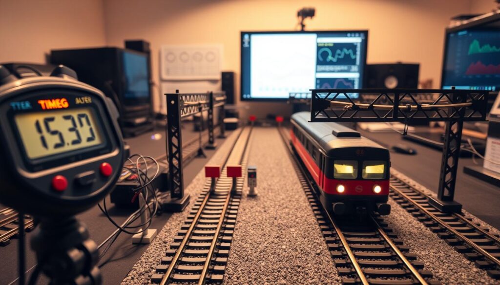
Calculating gives you average speed across the sensor span, not exact velocity. It’s like judging a sprinter by their overall race time instead of peak velocity. The closer your gates, the better your approximation.
One trial gives you something. Three trials tell you the truth. The wooden locomotive doesn’t roll the same every time—friction and wheels can slip. Running multiple trials isn’t excessive caution; it’s scientific methodology.
The TeachEngineering activity protocol shows proper experimental design. Students release trains from five different heights: 6, 12, 18, 24, and 30 centimeters. They perform three trials at each height. That’s 15 data points total, enough to calculate meaningful average speed values and identify patterns.
Recording measurements in organized tables isn’t busywork—it’s how scientists maintain integrity. Each trial gets its own row, each measurement its own column. Suddenly, you’re building a dataset that reveals relationships between energy types.
But let’s address the elephant on the tracks: instantaneous speed versus average velocity. True instantaneous speed requires measuring velocity at a single point in time. This is calculus territory, and unless you’re ready to discuss limits approaching zero, we’re capturing excellent approximations instead.
For classroom purposes, these approximations work beautifully. If your gates are close enough that the train hasn’t accelerated or decelerated significantly between them, you’re measuring something remarkably close to true velocity at that track position. It’s the difference between a snapshot and a short video clip—both capture reality, just at different resolutions.
Statistical analysis emerges naturally from multiple trials. Calculate the mean of your three runs, determine the range of variation, and suddenly you’re discussing experimental uncertainty like a proper scientist. Students learn that measurement variation isn’t failure—it’s reality, and accounting for it strengthens conclusions.
| Release Height (cm) | Trial 1 Speed (m/s) | Trial 2 Speed (m/s) | Trial 3 Speed (m/s) | Average Speed (m/s) |
|---|---|---|---|---|
| 6 | 0.89 | 0.92 | 0.88 | 0.90 |
| 12 | 1.24 | 1.28 | 1.26 | 1.26 |
| 18 | 1.51 | 1.48 | 1.53 | 1.51 |
| 24 | 1.73 | 1.76 | 1.71 | 1.73 |
| 30 | 1.91 | 1.95 | 1.93 | 1.93 |
The table above shows typical data collection results from a complete experimental run. Notice how speeds increase with release height—exactly what physics predicts when converting gravitational energy into kinetic energy. The trial-to-trial variation stays small but measurable, demonstrating both experimental consistency and natural variability.
This systematic approach transforms abstract physics concepts into tangible numbers. Students aren’t memorizing formulas; they’re discovering relationships through direct measurement. When they see speed increasing predictably with height, they’re witnessing energy conservation in action, not just reading about it in a textbook.
Scale conversion mph kph quick calculator and ratio table
Ever wonder what 0.5 mph means in a 1:87 world? Welcome to the world of scale conversion. Here, your model train’s slow pace becomes a high-speed thrill in miniature. The math is simple, but it’s mind-bending.
First, measure your train’s speed in real life. Then, multiply it by your scale ratio. For example, if your HO scale speed is 0.5 mph, multiply by 87. This gives you 43.5 mph. That’s faster than most speed limits and could get you a ticket.
Different scales give different results. N scale is 1:160, making 0.5 mph equal 80 scale mph. That’s very fast. O scale is 1:48, making 0.5 mph equal 24 scale mph. This feels more real.
But, there’s an international twist. Americans use mph, while Europeans use kph. The conversion factor is 1.60934. Multiply any mph by this to get kph. A quick trick: 100 kph is about 62 mph.
A ratio table saves you from calculator trouble. List speeds, apply scale factors, and see if your train is realistic or too fast:
| Measured Speed (mph) | HO Scale (1:87) mph | N Scale (1:160) mph | O Scale (1:48) mph | HO Scale (kph) |
|---|---|---|---|---|
| 0.25 | 21.75 | 40.0 | 12.0 | 35.0 |
| 0.50 | 43.5 | 80.0 | 24.0 | 70.0 |
| 0.75 | 65.25 | 120.0 | 36.0 | 105.0 |
| 1.00 | 87.0 | 160.0 | 48.0 | 140.0 |
| 1.50 | 130.5 | 240.0 | 72.0 | 210.0 |
Creating a chart for your model railroad scale makes every timing session easy. No more calculator trouble. Just check your chart to see if your train is realistic or too fast.
Do you want operational realism or visual realism? Operational realism means matching real speeds. Visual realism means making it look right. Sometimes, these don’t match, and model railroading becomes art.
The speed that calculates perfectly might look wrong. Our brains see motion differently at model scale. A train might look slow because we’re watching from a giant’s view. Many run 25-30% slower than calculated to look more realistic.
This creates a dilemma. Do you report the mathematically correct speed or acknowledge the gap between calculation and observation? Both answers are valid. One satisfies the math; the other satisfies the eye. Welcome to the world where numbers and aesthetics clash.
Plot distance time and velocity time curves area under curve distance
Collecting data is rewarding, but seeing it plotted reveals patterns that turn numbers into physics poetry. Graphs show motion in a way numbers alone can’t. They unlock secrets that data alone can’t.
Your distance time graph tells the first chapter of this story. Plot time on the horizontal axis and distance traveled on the vertical. Watch what emerges when you connect those data points.
The curve starts flat when your train sits at rest. Then it bends upward as the locomotive accelerates down the track. That increasing steepness isn’t random—it’s the visual signature of kinematics in action.
Here’s where calculus hides in plain sight: the slope of your distance time graph at any point equals instantaneous velocity. Steeper slope means higher speed. A flat section means the train stopped at the station. This connection between graphical slope and physical velocity is fundamental to understanding motion.
For trains accelerating down an incline, you’ll see a parabolic curve. That distinctive shape appears everywhere in physics—from falling apples to launching rockets. It’s the mathematical fingerprint of constant acceleration, and you just captured it with timing gates and model trains.
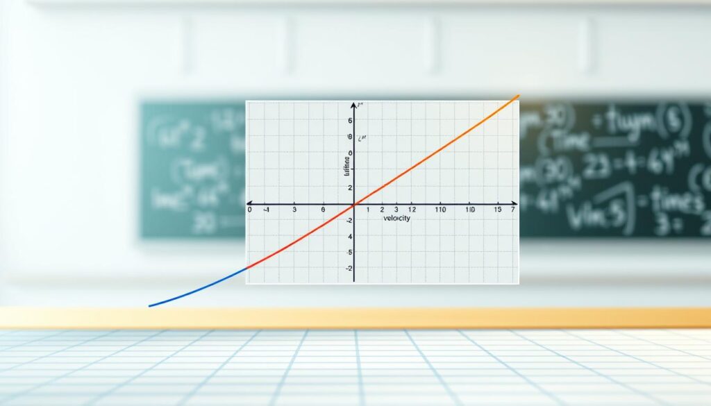
Now flip to your velocity graph. Plot time horizontally again, but this time put velocity on the vertical axis. For accelerating motion, you’ll see a straight line climbing upward—constant acceleration produces linear velocity increase.
Here’s the party trick that makes physics teachers weep with joy: the area under that velocity-time curve equals total distance traveled. You’re doing integration without calling it integration. Geometry reveals physics, and suddenly calculus makes visceral sense.
Compare both graph types side by side to see how they complement each other:
| Graph Type | Vertical Axis | Slope Represents | Area Represents |
|---|---|---|---|
| Distance-Time | Position (meters) | Instantaneous velocity | Not physically meaningful |
| Velocity-Time | Speed (m/s) | Acceleration rate | Total distance traveled |
| Constant Speed | Straight diagonal line | Horizontal straight line | |
| Acceleration | Upward parabolic curve | Upward sloping line |
The NGSS standard MS-PS3-1 requires students to construct and interpret graphical displays. These graphs show relationships between kinetic energy, mass, and speed. They deliver exactly that educational objective while documenting real experimental data from your layout.
Follow these steps to create your kinematics graphs:
- Transfer your timing data into graphing software or graph paper—Excel, Google Sheets, or Desmos work perfectly
- Create your distance-time plot first, marking each timing gate position against the time recorded
- Draw a smooth curve through your data points—resist the urge to connect them with straight lines
- Generate your velocity-time plot using your calculated speeds from each segment
- Calculate the area under your velocity curve using geometric shapes or numerical integration to verify it matches your total distance
You’re not just measuring speed anymore. You’re documenting the fundamental laws governing motion in our universe. That’s speed visualization with intellectual weight.
And if watching abstract numbers transform into elegant curves revealing Newton’s laws doesn’t make you feel like Galileo with better toys, check your pulse. This is where hobby becomes science, where play becomes discovery.
Challenge braking zone measure decel stopping distance vs speed
Every model train project needs a villain, and today that villain is uncontrolled kinetic energy barreling toward a scale platform. You’ve mastered measurement. You’ve conquered conversion. Now comes the truly exciting physics challenge: designing a braking system that transforms momentum into a gentle stop without sending imaginary passengers through the windshield.
The challenge sounds deceptively simple. Slow your runaway train to a comfortable final velocity using only available materials and the laws of physics. Suddenly you’re not just observing motion—you’re manipulating it, bending Newton’s first law through creative application of friction, drag, or mechanical resistance.
Here’s where things get mathematically spicy. The relationship between initial model train speed and braking distance isn’t linear—it’s quadratic. Double your entry velocity and you need four times the distance to achieve the same stop. This exponential relationship explains why highway engineers lose sleep and why your locomotive doing 43.5 scale mph needs serious intervention before impact.
Understanding stopping distance requires grasping deceleration as negative acceleration. When you apply brakes, you’re introducing forces that oppose motion—friction between brake pads and wheels, air resistance against surfaces, or magnetic fields inducing opposing currents. Each mechanism follows different physical principles but achieves the same goal: converting kinetic energy into heat or other forms.
Students get beautifully inventive with braking solutions. Past projects have featured foam bumpers, friction strips made from sandpaper, magnetic braking systems, and yes—tiny parachutes deployed at the critical moment. Each approach teaches different physics concepts and engineering trade-offs.
The measurement methodology reverses your timing gate setup. You know the entry model train speed from your previous calculations. You measure the braking distance from brake activation to complete stop. With those two data points, you can calculate average deceleration using kinematic equations.
The math transforms abstract formulas into tangible design constraints. Using the equation v² = u² + 2as, you determine acceleration (negative for braking) from initial velocity (u), final velocity (v = zero at rest), and distance traveled (s). Rearranging gives you: a = -u² / 2s. That negative sign indicates deceleration—the rate at which velocity decreases.
Will your brake stop a train released from 30 cm as effectively as one from 15 cm? The physics says absolutely not—unless you engineer variable resistance that responds to velocity. Advanced designs might incorporate progressive braking that increases friction as speed rises, similar to how real trains use regenerative braking systems that improve motion realism while recovering energy.
Real-world applications abound in this exercise. Train braking systems must account for loaded versus empty cars, wet versus dry rails, and emergency versus scheduled stops. Automotive safety engineers calculate stopping distance based on speed, road conditions, tire quality, and brake temperature. Understanding these relationships saves lives.
| Braking Method | Physics Principle | Effectiveness | Design Complexity |
|---|---|---|---|
| Foam Bumper | Compression resistance converts kinetic energy to deformation | Moderate for low speeds | Low – simple installation |
| Friction Strip | Surface texture creates opposing force proportional to normal force | High – consistent deceleration | Medium – requires surface preparation |
| Magnetic Brake | Eddy currents in conductor oppose magnetic field motion | Very high – velocity dependent | High – requires magnets and conductive material |
| Air Resistance | Drag force increases with velocity squared | Low for model scales | Medium – requires deployment mechanism |
Testing multiple entry speeds reveals how stopping distance scales with initial velocity. Create a data table comparing release heights (which determine entry speed) against measured braking distances. Plot these values and you’ll see that beautiful parabolic relationship emerge—visual proof that v² matters more than v.
The most sophisticated student projects incorporate sensors that measure deceleration in real-time. By placing timing gates at intervals through the braking zone, you capture velocity at multiple points and calculate instantaneous deceleration rates. Does your friction brake provide constant deceleration, or does it vary as materials compress or heat up?
This physics challenge elevates your project from passive observation to active engineering. You’re not just measuring what happens—you’re designing what happens, predicting outcomes through calculation, then validating predictions through experimentation. That’s the scientific method in action, powered by a model train and some creative friction.
Error sources reaction time sensor lag wheel slip rounding
Every measurement has a hidden margin of error. Your timing gate with its Arduino brain and aluminum foil sensors gives you data. But, that data comes with uncertainty, like a surprise gift.
If you expect perfect precision from simple materials, you might be disappointed. Measurement error hides in every reading, like a sneaky stowaway.
Sensor lag is a big problem. The photo interrupter doesn’t react right away when the beam breaks. This delay, though small, can affect your measurements a lot.
Wheel slip is another issue. During quick starts, the wheels might spin without moving forward much. This means your distance calculations might not be right.
Using aluminum foil adds its own set of problems. Sometimes, the foil doesn’t make good contact, thanks to poor sensor quality. Oxidation and inconsistent contact are common issues.
Common errors in model train timing include:
- Sensor response delay – photodiodes and contact switches introduce lag between event and detection
- Clock resolution limits – microcontroller timing precision constrains measurement granularity
- Mechanical slip – wheels spinning without traction during acceleration or braking
- Rounding artifacts – truncating decimals during unit conversion or display
- Track surface variation – inconsistent friction across different segments
- Environmental factors – temperature affecting electrical resistance and wheel grip
Hardware limits can make things worse. The distance between gates affects how accurate your measurements are. The surface of your track can also change, and the weight of your train can vary.
| Error Category | Typical Magnitude | Mitigation Strategy | Impact on Results |
|---|---|---|---|
| Sensor lag | 2-5 milliseconds | Calibrate with known speeds | Systematic bias in timing |
| Wheel slip | 5-15% during acceleration | Use constant velocity segments | Overestimated speed values |
| Rounding errors | 0.1-0.5% cumulative | Maintain extra decimal places | Random variation in calculations |
| Contact inconsistency | 10-30% detection failure | Multiple trial averaging | Missing data points |
Rounding errors sneak up on you. They happen when you convert units or display results on small screens. These small changes can add up and affect your results.
Understanding errors is key. They’re not just mistakes; they’re part of the real world. Science is about facing these imperfections head-on.
Instead of saying you measured exactly 2.00 m/s, say 2.0 ± 0.1 m/s. This shows you know about the uncertainty. It’s important to understand where errors come from and design experiments to minimize them.
This is what makes science real. Measurement error is not the enemy; it’s what makes science honest.
Extension schedule a mixed stop commuter service to the minute
Creating a commuter schedule is more than just knowing train speeds. It’s about precise timing across the whole route. Realistic operations turn your physics test into a real transportation system. You’re not just measuring speed; you’re managing a whole railroad.
Real railroads deal with big math problems every day. Train dispatchers figure out travel times between stations. They also consider acceleration zones, braking distances, and how long trains stay at stations.
Your extension project shows this complexity on your model layout. You’ll plan a schedule with express trains that skip stops and local trains that stop at every station. The physics you learned earlier helps plan these operations.
Begin by breaking your route into segments. Each segment needs a distance and a max scale mph rating. Express trains might go 60 scale mph over long distances, while locals go 15 scale mph through station zones.
Calculate the average speed for each train type over the whole route. Express trains go faster because they don’t stop as much. Local trains spend a lot of time slowing down and speeding up, which lowers their average speed.
Now, the math gets harder. If your morning express needs to arrive at Union Station at 8:15 AM, you must work backward. You need to account for every slow part of the route.
| Schedule Element | Time Required | Mathematical Basis |
|---|---|---|
| Segment travel time | Distance ÷ speed | Basic velocity equation |
| Station dwell | 30-60 seconds per stop | Fixed operational requirement |
| Braking approach | 10-15 seconds | Deceleration from previous section |
| Acceleration departure | 10-15 seconds | Reaching line speed |
A sample calculation shows the complexity. Your express covers 8 scale miles at 60 scale mph, needing 8 minutes to travel. Add a 45-second station stop, plus 20 seconds for braking and acceleration.
The next segment is 4 scale miles at 30 scale mph, taking another 8 minutes. Suddenly, your simple speed test turns into complex train scheduling math that adds up across the whole route.
Model railroad operations need to track timing errors. Small delays can add up. A train 30 seconds late at station two might be 2 minutes behind by station five, thanks to slower traffic ahead.
Design your schedule using these categories:
- Express service: Few stops, higher average speed, simpler speed profiles with fewer speed changes
- Local service: Stops at every station, constant speed changes, complex timing needs across many stations
- Mixed operation: Some trains pass others, needing careful schedule planning to avoid conflicts
Use a spreadsheet to track each train’s progress minute by minute. List every station, the scheduled arrival time, dwell time, and departure time. Use your speed data to calculate travel times to the next station.
The joy comes when everything works perfectly. Your 8:02 local departs on time, stays on schedule through five stops, and arrives at the end at 8:34—just as planned. That’s transportation engineering in miniature.
Challenge yourself with tough goals. Can you schedule an express to pass a local without either train waiting at a station? What if you add a freight train that blocks the mainline for a long time?
This extension turns your layout into a real system. Realistic operations mean physics helps practical goals. Your speed measurements help schedule trains precisely, and your timing accuracy decides if passengers (imaginary though they may be) reach their destinations on time.
You’re not just playing with trains anymore. You’re managing a network where math meets logistics, and every second matters. Welcome to the world of train scheduling—it’s tougher than it seems, but incredibly rewarding when you get it right.
Student report template graphs tables discussion prompts
Documentation is key in science, separating real findings from just guesses. The student project report template helps turn simple observations into meaningful science. It shows that “we watched trains go fast” actually means something.
Begin with the hypothesis section. Here, students guess what will happen before they collect data. Will trains go twice as fast if the track is twice as long? Recording these guesses teaches students to own up to their mistakes. Saying “I was completely wrong” is a valid scientific finding.
Data tables help make sense of messy data. They organize information into neat rows and columns. This makes sure the data is reliable across different tests. The distance time graph shows patterns that random drawings can’t.
Discussion prompts take the report to the next level. They ask deeper questions like why speed increases with height. What does the graph’s slope mean? What errors might have affected the results? How might this apply in real-world engineering?
This template is not just busywork. It helps students turn their experience into real understanding. It turns simple observations into deep insights. Science is about asking good questions and documenting the journey to knowledge.
And sometimes, it’s about trains. Those amazing, precisely-timed, mathematically-optimized trains.
