
Opening your textbook and feeling dread is normal. Thermodynamics doesn’t have to be as hard as building IKEA furniture in the dark.
This guide makes students who want to build things understand thermodynamics better. We focus on energy bookkeeping that makes sense and steam tables that are easy to read.
Sadi Carnot figured out the basics in 1824 while improving steam engines. The main challenge is understanding how heat turns into work. You also need to track energy transfer and why efficiency is important. The first law is your foundation.
This field is important for many things, like power plants and refrigerators. Classical thermodynamics helps us understand systems at near-equilibrium. It uses measurable properties to model work and heat exchanges.
Let’s learn thermodynamics in a clear and practical way. We’ll do it with a bit of fun and a nod to those who made it too hard.
First law applied to boiler and cylinder work output
Heat engines have a strict rule: every joule must be accounted for. The first law of thermodynamics is like a strict accountant. It makes sure energy conservation is followed, not just suggested.
You can’t just create energy out of thin air. And you can’t make it vanish. All you can do is change its form.
Take a steam engine, for example. It’s a classic heat engine. We track every bit of energy it uses. Heat goes into the boiler, which is your Qin.
Some of that heat stays in the system, raising its internal energy. The rest is what makes the piston move and does work. That’s your Wout.
The math is simple: ΔU = Q – W. This means the change in internal energy is the heat added minus the work done. Notice, it’s about changes, not fixed values.
This simple formula often confuses students. They remember it but miss the big picture. Internal energy is about the state of the system, not how it got there.
Heat and work, on the other hand, depend on the path. They show how energy moves across the system boundary.
Let’s look at a real example. Your boiler heats water to make steam. This steam then pushes a piston in a cylinder. The piston does work as it moves.
Heat goes in, and work comes out. The difference is the change in the system’s internal energy. It’s basic, right?
But real systems are complex. They lose heat and energy to friction. Yet, the first law remains true. Every joule goes somewhere, even if it’s wasted.
Sign conventions are key. Positive Q means heat in, and positive W means work done by the system. Get these wrong, and your math will fail fast.
Keep track of your energy flows carefully. Mark heat entering the boiler as positive. And mark work done by the piston as positive too. The energy conservation rule doesn’t care about your confusion—it just demands balance.
Understanding this energy balance is the key to grasping all heat engines. The math is straightforward. But visualizing energy flow is what trips up students.
Enthalpy and steam tables how to read hf hg hfg examples
Thermodynamics is like a language, and steam tables are its dictionary. Enthalpy is a key term that might seem tricky at first. But once you get it, these tables become your go-to tool.
Enthalpy is a mix of internal energy and the work needed to fit your substance into the world. It’s calculated as H = U + PV, where U is internal energy, P is pressure, and V is volume.
Why is this important? Because fluids in real systems, like boilers and turbines, usually work at constant pressure. In these cases, enthalpy changes show how much energy is being moved.
Now, let’s look at the symbols in steam tables. You’ll see three main ones:
- hf – enthalpy of saturated liquid (water at the brink of boiling)
- hg – enthalpy of saturated vapor (pure steam, no liquid droplets)
- hfg – the difference between them, representing latent heat of vaporization
The last one, hfg, shows the energy needed for phase change. It’s the energy that turns liquid to gas without changing temperature. This energy is what powers steam engines and makes your kettle whistle.
Here’s how to use them. Find your pressure or temperature in the leftmost column. Then, slide your finger across the row to find the corresponding thermodynamic properties.
Working with wet steam? That’s steam that’s part liquid, part vapor. You’ll need to know the quality, denoted as x, which shows the vapor fraction.
The formula is simple: h = hf + x · hfg. For example, if you have steam at 100°C with quality x = 0.8, you’re dealing with 80% vapor and 20% liquid droplets.
| Property | Symbol | Value at 100°C | Units |
|---|---|---|---|
| Saturated liquid enthalpy | hf | 419.04 | kJ/kg |
| Evaporation enthalpy | hfg | 2257.0 | kJ/kg |
| Saturated vapor enthalpy | hg | 2676.0 | kJ/kg |
| Wet steam (x=0.8) | h | 2224.6 | kJ/kg |
Try it yourself: 419.04 + (0.8 × 2257.0) = 2224.6 kJ/kg. See? The numbers make sense once you know the formula.
This science didn’t start yesterday. Professor Joseph Black at the University of Glasgow discovered heat capacity and latent heat in the 1700s. He found that ice melting or water boiling absorbs a lot of energy without changing temperature. This discovery started the field of thermodynamics.
We’ve been making these steam tables ever after, organizing decades of data into rows and columns. They might look scary at first. But with practice, they become as easy as reading sheet music.
Your calculator and these tables are your best friends for thermodynamic calculations. Learn to use them well, and you’ll be a pro at sizing boilers or analyzing power cycles. The symbols will become clear in no time.
PV and TS sketches indicator cards work as loop area
In 1738, Daniel Bernoulli was sketching particles bouncing off pistons. He didn’t know he was inventing the language of engines. His drawings were the start of powerful visual tools in thermodynamics.
Thermodynamics gets visual, and it’s about time. PV diagrams show pressure versus volume. TS diagrams plot temperature against entropy. They are like graphic novels of thermodynamics, telling the story without equations.
The key insight is work is area. On a pressure-volume graph, the area under a curve shows work during a process. The area enclosed by a complete loop is your net work output per cycle.
This isn’t abstract math doing gymnastics. It’s geometry doing physics, and it’s practical. Sketching thermodynamic cycles on PV diagrams shows the path of your working fluid.
The journey has four basic movements. Compression pushes work into the system. Heating causes volume expansion. Expansion pulls work out of the system. Cooling reduces volume back to the start.
The loop closes because cycles repeat. Bigger loop? More work per cycle. It’s simple and profound.
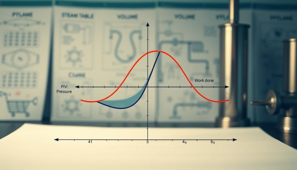
In the 1800s, engineers used indicator cards to draw PV diagrams of operating engines in real-time. These weren’t theoretical sketches; they were direct measurements of actual engine performance.
A spring-loaded pencil tracked piston motion on one axis. Cylinder pressure pushed the pencil on the other axis. This gave an instant visual record of engine performance.
TS diagrams tell a parallel story with temperature and entropy as the axes. Here too, area equals heat transfer. Different processes are clearer on different plots.
| Process Type | PV Diagram Appearance | TS Diagram Appearance | Key Insight |
|---|---|---|---|
| Isothermal (constant temperature) | Curved hyperbola | Horizontal line | Heat equals work done |
| Isentropic (constant entropy) | Steep curve | Vertical line | Adiabatic and reversible |
| Isobaric (constant pressure) | Horizontal line | Curved line upward | Volume changes with heat |
| Isochoric (constant volume) | Vertical line | Curved line varying | Pressure changes with heat |
It’s like looking at a building’s floor plan versus its elevation view. Same structure, different perspectives. Each reveals details the other hides.
Isothermal processes are horizontal lines on TS diagrams but curves on PV diagrams. Isentropic processes are vertical on TS, curves on PV. Master both, and you’ve got stereoscopic vision for heat engines.
The practical value here can’t be overstated. These diagrams aren’t just pretty pictures for textbooks. They’re diagnostic tools that reveal inefficiencies, lost work, and optimization opportunities at a glance.
When your actual indicator card doesn’t match your theoretical cycle diagram, you’ve found your problem. Maybe there’s pressure drop in the valves. Maybe combustion isn’t complete. Maybe heat loss is greater than calculated. The diagram shows you where reality diverges from theory.
Learn to sketch these quickly and accurately. Start with the Rankine cycle, then move to Otto, Diesel, and Brayton cycles. Draw them on both coordinates. Watch how work manifests as loop area every single time.
This visual intuition separates thermodynamics students from practitioners. You’re not just calculating numbers anymore. You’re seeing energy transformation happen. You’re watching work emerge from heat, compression transform into motion, and cycles complete their eternal loops.
Daniel Bernoulli’s particle sketches from 1738 presaged this entire approach. He understood that sometimes you need to draw what’s happening before you can calculate it. The equations came later; the vision came first.
Simple Rankine boiler engine condenser pump losses
Welcome to the Rankine cycle, where thermodynamics meets the real world of heat engines. It’s a model that shows how steam power plants work. It’s key to understanding over a century of electricity.
The cycle starts with the boiler adding heat, turning water into steam. This steam then expands through an engine or turbine, doing work. The steam then goes to a condenser, where it cools down and turns back into liquid. A pump then pushes this liquid back to the boiler, starting the cycle again.
Real Rankine cycle systems lose energy at every step. The boiler loses heat, and the turbine faces friction. The condenser can’t perfectly reject heat, and the pump isn’t 100% efficient.
James Watt improved steam engines in 1776, tackling these efficiency losses. His work helped start the Industrial Revolution. William Rankine wrote the first thermodynamics textbook in 1859, highlighting the gap between theory and reality.
The gap between ideal and real performance is where engineering shines.
When calculating Rankine cycle efficiency, start with the ideal. Then, add losses from real equipment. Here’s what that looks like:
| Loss Source | Typical Penalty | Impact on Efficiency |
|---|---|---|
| Turbine inefficiency | 4-6% | Friction and blade losses |
| Condenser approach | 2-4% | Temperature difference required |
| Pump work | 1-3% | Mechanical and fluid friction |
| Boiler heat loss | 3-5% | Radiation and convection |
So, your 38% ideal efficiency drops to 28% actual. That 10-point gap is where mechanical engineers find their work. Every percentage point saved means millions in fuel costs for power plants.
Understanding these efficiency losses isn’t pessimism. It’s a realistic view, where innovation thrives. The Rankine cycle gives you a framework. Real systems teach you the value of improvement.
Hands on pop can engine where is heat where is work
A soda can, some wire, and a flame teach more about heat engines than any lecture. You feel the power of thermal energy when you see your creation move.
The pop-can engine is simple. It uses aluminum, water, and heat. It’s like a song of thermodynamics, easy to understand.
Heat from your flame goes into the can’s bottom. It turns the water inside into vapor. This vapor pushes against a piston, making it move.
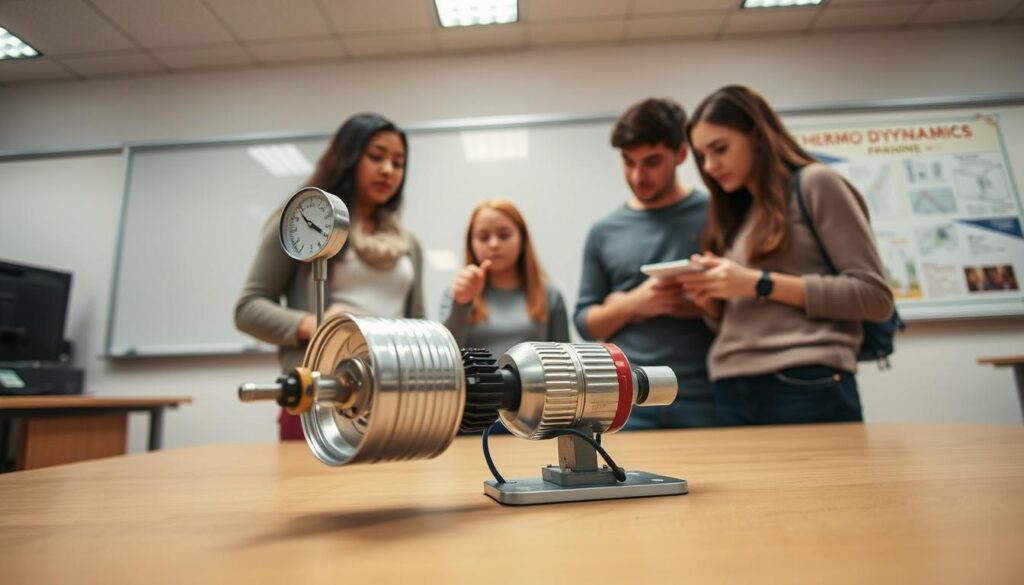
Heat enters the system through the can’s wall. It warms the water molecules, making them move faster. You can feel this if you touch the can.
Work is done at the piston. The expanding vapor pushes against it. This turns thermal energy into motion, showing the first law in action.
Simulation tools like AxSTREAM help students model systems quickly. But nothing beats the real experience of working with hot aluminum.
Thermodynamics devices have been around for ages. Hero’s engine used steam to spin a sphere. The pop-can engine shows the same basic idea.
Build your engine and measure everything. Use fuel consumption and combustion enthalpy to calculate heat input. Attach weights to measure work output. Then, calculate efficiency.
Your efficiency will likely be low, around 2-5%. But that’s where the learning starts. You’ll see why losses happen.
| Energy Flow | Location | Observable Effect | Typical Loss % |
|---|---|---|---|
| Heat Input | Flame to can bottom | Water temperature rise, bubbling | 40-50% escapes to air |
| Phase Change | Liquid to vapor inside can | Pressure increase, can bulging | 20-30% incomplete vaporization |
| Mechanical Work | Vapor pressure on piston | Visible motion, weight lifting | 15-25% friction losses |
| Heat Rejection | Condensation, ambient cooling | Vapor returning to liquid | Remaining energy dissipated |
You’ll see every loss mechanism in action. Heat escapes to air instead of water. Friction and incomplete combustion also play a role.
This isn’t just a classroom trick. It’s a test of your engineering skills. You’ll appreciate the efficiency of real power plants more.
Building a working engine is more than just knowing about practical thermodynamics. It’s about understanding it deeply.
This hands-on experience is invaluable. You learn about energy flows and why efficiency matters. You see why small improvements are huge achievements.
Ancient inventors learned through trial and error. You have the advantage of theory. Explain why your pop-can engine works using the first law and thermodynamics.
Combining hands-on building with theory changes you. You go from passing a test to truly understanding thermodynamics. Build, measure, and appreciate the hard work of real engineers.
Estimate work per cycle using pavg × ΔV numbers
Ever seen an engineer quickly come up with a number that saves hours of work? That’s the power of estimation. The formula is simple: W ≈ Pavg × ΔV. Work per cycle equals average pressure times volume change. This quick calculation can make a big difference in getting things done.
Why does this work? Work is the integral of pressure with respect to volume. For complex curves, that means using calculus. But if you can estimate average pressure, you can get work output pretty close.
Is it good enough for initial studies? Absolutely.
Let’s look at an example. An engine cylinder expands from 50 cm³ to 500 cm³. That’s a volume change of 450 cm³. Pressure starts at 10 bar and drops to 2 bar. What’s the work?
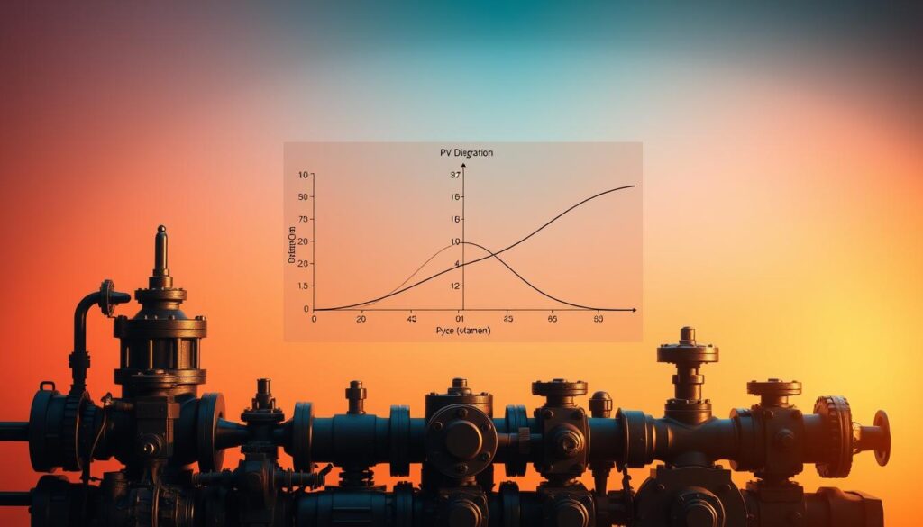
The average pressure isn’t just the mean of 6 bar. For adiabatic expansion, it’s about 0.6 times the initial pressure. So, Pavg ≈ 6 bar. Now, the calculation is easy: W ≈ 6 bar × 450 cm³ = 2,700 bar·cm³ = 270 J per cycle.
That’s your work output. At 3,000 RPM, that’s 13,500 watts or about 18 horsepower. From a simple multiplication.
Estimating Pavg correctly is key. Different processes need different approaches. Understanding the process is more important than your calculator.
| Process Type | Pavg Estimation Method | Typical Accuracy | Best Application |
|---|---|---|---|
| Isothermal Expansion | Pavg = (P₁ – P₂) / ln(P₁/P₂) | ±5% | Slow compression cycles |
| Adiabatic Expansion | Pavg ≈ 0.6 × P₁ | ±12% | Fast engine strokes |
| Polytropic (n=1.3) | Pavg = (P₁ – P₂) × n/(n-1) | ±8% | Real gas processes |
| Constant Pressure | Pavg = P₁ = P₂ | ±2% | Boiler heating |
This method works because engines usually operate in narrow ranges. It’s the 80/20 rule in thermodynamics. When you’re designing, this approach is invaluable.
It’s also a sanity check for your detailed simulations. When your calculator dies, this might save you. Learn the formal integration methods, absolutely—but master this approximation for real-world use.
The beauty of this method? You can sketch pressure-volume relationships anywhere and get good estimates. That’s not laziness. That’s engineering judgment in action.
Efficiency vocabulary thermal mechanical overall improvements
What sets apart the top thermodynamics students? It’s their grasp of efficiency vocabulary. This isn’t just theory; it’s where thermodynamics meets economics. Suddenly, everyone from your boss to investors wants to know your numbers.
But beware, there are many efficiency definitions. Getting them mixed up can lead to wrong answers and awkward meetings.
Let’s focus on the key terms.
Thermal efficiency (ηthermal) is key. It shows how well a heat engine turns thermal energy into work. The formula is simple: work output divided by heat input.
For a Rankine cycle, you use enthalpy changes: ηthermal = (hin – hout)/(hboiler_in – hpump_out). Simple cycles get about 25% efficiency. More complex ones can hit 45%.
Mechanical efficiency (ηmechanical) looks at real-world losses. Friction, bearings, and seals all play a part. It compares theoretical work to actual output.
A top turbine can reach 85-95% mechanical efficiency. That small engine from Section 6? It might get 30%, if you’re lucky.
Overall efficiency (ηoverall) is what matters most. It’s the product of thermal and mechanical efficiencies: ηoverall = ηthermal × ηmechanical. Even with 38% thermal efficiency, mechanical losses can cut it in half.
This number decides if your power plant makes money or loses it.
| Efficiency Type | Formula | What It Measures | Typical Range |
|---|---|---|---|
| Thermal | Wout / Qin | Thermodynamic cycle performance | 25-45% |
| Mechanical | Wshaft / Wcycle | Friction and parasitic losses | 30-95% |
| Overall | ηthermal × ηmechanical | Real-world system performance | 20-40% |
Improvements come in two types. Knowing which one you’re aiming for is key to avoiding costly mistakes.
Thermal efficiency improvements focus on the cycle itself:
- Raise the high temperature or lower the low temperature (Carnot’s fundamental insight)
- Add regenerative feedwater heating to recover waste heat
- Implement combined cycles that cascade through multiple working fluids
- Optimize pressure ratios and expansion paths
Mechanical efficiency improvements tackle physical losses:
- Reduce friction with better bearings and advanced lubrication
- Minimize flow losses through streamlined passages
- Optimize blade geometry in turbines
- Reduce auxiliary power consumption
The history of thermodynamics was driven by the quest for better steam engine efficiency. Sadi Carnot, James Watt, and William Rankine all worked to get more work from less fuel. Their efforts built empires and powered the Industrial Revolution.
Today, with energy costs rising and environmental rules tightening, efficiency is more critical than ever. A 2% efficiency boost in a 500 MW plant saves millions a year. It also cuts emissions, making everyone happy.
Efficiency isn’t just about numbers. It’s about understanding trade-offs. Higher efficiency often means spending more upfront. It’s about finding the bottlenecks in your system.
Most importantly, it’s about clear communication. Know which efficiency you’re talking about. A turbine maker might mean mechanical efficiency, while a power plant operator talks about overall efficiency.
Get these terms mixed up, and your proposals won’t help. Master the vocabulary, and you can talk about system performance with anyone.
That’s when thermodynamics turns from classroom theory into a career boost.
Extension Carnot limit why real engines are lower
The thermodynamic speed limit is not just a suggestion. It’s a hard limit set by physics. Every heat engine faces theoretical limits set by Sadi Carnot in 1824. His work, Reflections on the Motive Power of Fire, showed the maximum efficiency possible for any heat engine.
The formula for this limit is simple but strict: ηCarnot = 1 – Tcold/Thot. Temperatures must be in Kelvin. This limit is not up for debate.
Take a steam plant working between 600°C (873 K) and 40°C (313 K). The Carnot cycle efficiency would be 64.2%. But, real plants might only reach 38%. This shows the big gap between theory and reality.
Why can’t real engines reach the Carnot heat engine efficiency? Carnot’s cycle needs perfect reversibility. This means no friction, no heat transfer issues, and infinite time for each step. It’s a theoretical ideal, not something we can make real.
Real engines face many problems. Here are some:
- Heat transfer gradients: Moving heat requires temperature differences, which waste thermodynamic energy
- Friction everywhere: Bearings, fluid flow, and blade passages turn organized work into heat
- Time constraints: Fast processes lead to more losses than slow ones
- Pressure drops: Piping, valves, and flow restrictions lose energy constantly
- Incomplete combustion: Real fuel burning never perfectly converts chemical energy
The second law of thermodynamics explains these limits through entropy. Entropy always increases in real processes. Entropy generation shows how much irreversibility and lost work there is.
Each problem reduces theoretical performance. The enthalpy changes from steam tables already show these limitations. They connect the first law energy balances to real equipment behavior.
How big is the gap between theory and practice? Check this comparison:
| Temperature Range | Carnot Efficiency | Typical Real Efficiency | Efficiency Ratio |
|---|---|---|---|
| 873 K to 313 K (Steam plant) | 64.2% | 38% | 59% of Carnot |
| 1400 K to 300 K (Gas turbine) | 78.6% | 42% | 53% of Carnot |
| 500 K to 300 K (Low-temp engine) | 40% | 15% | 38% of Carnot |
Real plants usually hit 40-60% of their Carnot limit. This isn’t because of bad engineering—it’s physics. The Carnot cycle is an ideal, not a goal to reach.
Understanding this gap is key. When you analyze enthalpy changes and apply the first law to real cycles, you’re already working within achievable efficiency limits. The theoretical limits show where to focus improvement efforts.
Want to boost real engine efficiency? Raise the hot temperature or lower the cold temperature. For example, increasing Thot from 873 K to 923 K (50 K increase) raises the Carnot limit from 64.2% to 66.1%. Improving material science to handle higher temperatures is a big efficiency booster.
Here’s the practical wisdom: If someone suggests a heat engine better than the Carnot cycle, they’re likely wrong. The Carnot limit is a strict limit against thermodynamic dreams.
But, there’s room for innovation within these rules. The 20-30% gap between current practice and theoretical limits means billions in fuel savings. Your engineering skills are key here, not in breaking thermodynamic laws, but in reducing irreversibilities.
Problem set step by step steam table practice
It’s time to put your knowledge to the test. Grab your steam tables and a calculator. The key to mastering thermodynamics is practice.
Begin with simple tasks. Choose a pressure and temperature. Decide if your steam is saturated or superheated. Find the enthalpy. Write it down and check your answer. Do it again.
Next, calculate work output for a turbine expansion. Use h₁ minus h₂. Look up both states in your steam tables. The numbers will tell you the story.
Your next challenge is analyzing a complete Rankine cycle. You’ll need four state points and four steam table lookups. Plus, one efficiency calculation. This is where everything comes together.
Work on ten problems, then ten more. The more you practice, the more comfortable you’ll become. You’ll stop worrying about thermodynamics questions and start seeing patterns.
The steam tables are just data waiting for you to find meaning. Each problem builds your confidence. Each calculation strengthens your understanding of pressure, temperature, and enthalpy.
Real engineers solve problems systematically. They check their work and verify units. They also draw diagrams. Start practicing these habits now, and thermodynamics will become your tool, not an obstacle.
Your job isn’t just memorization. It’s about understanding how energy moves through systems and proving it through calculation.
